Unit 5: Operations management
5.6 Production planning
HL This subtopic is HL only. You are viewing SL content, so treat this page as extension material; switch to HL to set it as part of your course.
Study mode could not start. The page reads as usual.
Study mode
On this page
Section 01: What the IB course asks
The content statements for 5.6, in the platform's words, with the depth of teaching the guide sets (guide, from p. 34).
- The local and global supply chain process AO2
- Just-in-time (JIT) versus just-in-case (JIC) AO3
- Stock control charts: lead time, buffer stock, reorder level and reorder quantity AO2, AO4
- Capacity utilization rate AO2, AO4
- Defect rate AO2, AO4
- Labour productivity, capital productivity, productivity rate and operating leverage AO2, AO4
- Cost to buy (CTB) and cost to make (CTM) AO3, AO4
AO1 knowledge and understanding · AO2 application and analysis · AO3 synthesis and evaluation · AO4 a range of skills. A question can use a command term at its statement's level or below. The whole course.
Section 02: Why it matters
A business that makes things has to get the right materials to the right place at the right time, use its capacity well, keep faults to a minimum and decide what to make itself and what to buy in. Production planning is the set of tools for those decisions.
This HL subtopic covers the supply chain that feeds production, the choice between holding stock just in case and receiving it just in time, the stock control chart, and the measures managers use to judge operations: capacity utilization, the defect rate, productivity and operating leverage. It ends with the choice between making and buying. Several of these are calculations (AO4), but each result needs interpreting: a number on its own decides nothing.
By the end you can
- Explain how a local and a global supply chain work, and the risks of each.
- Evaluate just-in-time and just-in-case stock control, and judge which suits a given business.
- Construct and interpret a stock control chart using lead time, buffer stock, reorder level and reorder quantity.
- Calculate capacity utilization, the defect rate, labour and capital productivity, the productivity rate and operating leverage, and comment on the results.
- Recommend whether to make or buy, using the cost to make and the cost to buy alongside non-financial factors.
Section 03: The local and global supply chain
A supply chain is the sequence of businesses and activities that turns raw materials into a product in a customer's hands: growing or extracting the materials, making components, assembling the product, storing and transporting it, and selling it. Goods flow forward along the chain; information, such as orders, sales data and complaints, flows back.
Supply chain management is the work of coordinating that chain: choosing suppliers; agreeing prices, quality standards and delivery dates, often with penalties for late delivery; deciding what to make and what to buy; organizing transport and storage; and checking that suppliers meet the business's standards on working conditions and the environment. Customers judge a business by the whole chain, not only by its own part of it. A late component, a faulty part or a supplier's unsafe factory becomes its problem.
A local supply chain keeps most of its stages in one country or region. A global one spreads them across the world to reach lower costs, scarce materials or specialist skills.
- Strengths of a local chain
Short lead times; easy communication in one language and time zone; closer checks on quality and working conditions; lower transport costs and emissions; and a "made locally" story for marketing.
- Weaknesses of a local chain
Often higher costs, especially of labour; a smaller choice of suppliers; and some materials or skills may not be available locally at all.
- Strengths of a global chain
Lower costs from cheaper labour and suppliers' economies of scale; access to materials and expertise found elsewhere; and a wider choice of suppliers.
- Weaknesses of a global chain
Long lead times and high transport costs; exposure to disruption from storms, conflict, blocked shipping routes or pandemics; changes in exchange rates and tariffs; and harder checks on how suppliers treat their workers and the environment.
- Managing the chain well
Brings reliable deliveries, lower costs, flexibility when demand changes, consistent quality and a reputation for ethical sourcing. Technology helps, because shared data and tracking show where every order is.
- Building resilience
After a disruption, many businesses spread their orders across more suppliers, hold more stock of critical parts, or bring some production closer to home (reshoring, subtopic 5.4), accepting some extra cost in return for a chain that is harder to break.
Text description
A supply chain in six stages: raw materials, suppliers of components, the manufacturer, distribution through wholesalers and warehouses, retailers, and customers. Goods flow forward along the chain while information such as orders, demand data and feedback flows back. A local chain keeps the stages in one country or region; a global chain spreads them across countries, which can lower costs but lengthens lead times and adds risk.
Section 04: Just-in-time versus just-in-case
Businesses hold three kinds of stock: raw materials and components waiting to be used, work in progress, and finished goods waiting to be sold. How much to hold is a trade-off. Too little and production stops; too much ties up cash and space in goods sitting on shelves. The two approaches the guide names sit at either end.
Just-in-case (JIC) holds generous stocks, including a buffer, as insurance against late deliveries, faults or a sudden rise in demand. Just-in-time (JIT) holds as little as possible: materials arrive just as they are needed and products are made to order, so stock is used almost as soon as it arrives. JIT is a method of lean production (subtopic 5.3), because stock that sits waiting is a form of waste.
Neither is right for every business. The choice depends on how reliable the suppliers are, how predictable demand is, how costly a stock-out would be compared with the cost of holding stock, and the nature of the product: perishable or fashion goods favour JIT, while critical spare parts favour JIC.
- JIT gains
Lower storage, insurance and security costs; cash and space freed for other uses; less waste from damage, theft and goods going out of date; and problems are exposed quickly instead of being hidden behind piles of stock.
- JIT risks
Production stops if a single delivery is late; there is no stock to meet a sudden surge in demand; more frequent, smaller orders lose bulk discounts and raise ordering and delivery costs; and the whole system depends on suppliers being reliable.
- What JIT needs
Reliable suppliers, often close by; good communication and shared data with them; a flexible, multi-skilled workforce; and quality that is right first time, because there is no spare stock to replace faulty parts.
- JIC gains
Production and sales continue when deliveries are late or demand jumps; buying in bulk earns discounts and means fewer orders; and customers can be served at once from stock.
- JIC costs
Cash tied up in stock that could be used elsewhere, an opportunity cost that also weakens liquidity; storage, insurance and handling costs; and the risk of stock perishing, being stolen or going out of fashion.
- Mixing the two
Many businesses use JIT for cheap, easily replaced items from nearby suppliers and keep buffer stocks of critical parts with long or uncertain lead times.
Text description
Two charts of stock held over twelve weeks, on the same scale. Just in case: a large delivery every four weeks takes stock to 900 units, and it never falls below a buffer of 300, giving protection against late deliveries and surges in demand but tying up cash and space. Just in time: a small delivery every week brings 150 units that are used up by the end of the week, so little stock is held and less is wasted, but there is no cushion if a supplier is late.
Section 05: Stock control charts
A stock control chart plots the level of one stock item over time and is used to plan when to reorder and how much. Stock falls steadily as it is used, then jumps when a delivery arrives, giving a saw-tooth pattern. The guide names four terms the chart uses:
- Lead time: the time between placing an order and the goods arriving, ready to use.
- Buffer stock: the minimum stock kept in reserve for late deliveries or unexpectedly high usage. In a normal cycle each delivery arrives just as stock reaches this level.
- Reorder level: the stock level at which a new order is placed, high enough to cover usage during the lead time on top of the buffer.
- Reorder quantity: how much is ordered each time, which is the height of each jump on the chart.
The top of each tooth is the maximum stock level, the buffer plus the reorder quantity. The slope of the falling line shows the usage rate: the steeper the line, the faster stock is used.
To construct one, put time on the horizontal axis and units of stock on the vertical. Draw horizontal lines for the maximum stock, the reorder level and the buffer stock. Then draw the saw-tooth, falling at the usage rate from the maximum to the buffer and jumping back up by the reorder quantity, and mark where each order is placed and the lead time that follows. The Operations Floor lets you test a stock plan against late deliveries.
- What sets the buffer stock
How reliable suppliers are, how much usage varies, the length of the lead time, the cost of running out, the storage space available and how perishable the stock is. Businesses using JIT keep very little.
- What sets the reorder quantity
Bulk discounts and the cost of placing orders, which favour large orders, against storage space, holding costs, the cash tied up and shelf life, which favour small ones.
- What a stock-out costs
Lost sales and perhaps lost customers, idle workers and machines, and the extra cost of rush deliveries. The buffer stock exists to make a stock-out unlikely, not impossible.
- A common confusion
The reorder level says when to order; the reorder quantity says how much.
Text description
Stock control chart over 12 weeks. Stock falls steadily from a maximum of 1,000 units at 200 units a week. An order is placed when stock reaches the reorder level of 600 units, the buffer stock of 200 plus 2 weeks of usage. The order of 800 units, the reorder quantity, arrives after the 2-week lead time, just as stock reaches the buffer stock, taking stock back to the maximum. The cycle repeats every 4 weeks.
Reorder level
Reorder level = buffer stock + (usage per period × lead time in periods)
The standard form; the guide gives no formula. Measure usage and lead time in the same periods, for example weeks.
Maximum stock level
Maximum stock level = buffer stock + reorder quantity
The standard form. It holds when each delivery arrives just as stock reaches the buffer.
Advantages
- Shows at a glance when to order and how much, and how long the business can last if a delivery is late.
- Makes the trade-off between the cost of holding stock and the risk of running out visible and easy to discuss.
Limitations
- Assumes stock is used at a steady rate, although demand varies by day and by season.
- Assumes the lead time is fixed and every delivery complete, which one late or short delivery breaks.
- Shows one item at a time, so a business with thousands of items needs software that reorders automatically.
Section 06: Capacity utilization
Productive capacity is the most a business can produce in a period with the resources it has now: its buildings, machines and staff. It is measured in units that suit the business, such as bikes a week, seats a night or patients a day. The capacity utilization rate shows how much of that capacity is actually being used.
The rate matters because fixed costs have to be paid whatever the output. The more of its capacity a business uses, the more units share the fixed costs, so the lower its cost per unit and the better its margins.
That does not make 100% the goal. A business working flat out has no room for maintenance, breakdowns or a rush order from a good customer; staff may be overstretched and quality may slip. Most businesses aim for a high rate with some room to spare. Explore the effect of output on cost per unit on the Operations Floor.
- Low utilization
Idle machines and staff push up the fixed cost of each unit. The business can try to boost demand through marketing or lower prices; use the spare capacity to make products for other businesses, or rent it out; or, if the fall in demand looks permanent, rationalize by closing sites, selling equipment or cutting staff.
- Demand above capacity
Customers have to wait or go elsewhere. The business can add overtime or extra shifts; subcontract work to other firms, at some risk to quality and margins; raise its price to ration demand; or invest in more capacity if the demand looks likely to last.
- Temporary or lasting?
A short dip or a seasonal peak may need no response at all; only a lasting change justifies changing the capacity itself.
Capacity utilization rate
Capacity utilization rate = actual output ÷ productive capacity × 100
As in the guide's formula list (p. 65).
Section 07: Defect rate and productivity
Four more measures show how well operations turn inputs into good output: the defect rate and three measures of productivity.
The defect rate is the share of the units made that fail to meet the required quality standard. Defects cost money twice: once to scrap or rework the faulty units, and again if any reach customers, through returns, complaints, recalls and damage to the brand. Cutting the defect rate is a main aim of quality management (subtopic 5.3).
Productivity measures output against the inputs used to produce it. Labour productivity is output per worker, or per hour worked; capital productivity is output per unit of capital, such as per machine or per machine hour. The guide's productivity rate compares total output with total input and multiplies by 100. For the percentage to mean something, value both in the same currency: output at its selling price and inputs at their cost.
Higher productivity lowers the cost of each unit and can pay for higher wages without higher prices. It can be raised through training, better equipment and technology, better methods and better motivation. Pushing it too hard has costs: rushed work can raise the defect rate, and long hours and pressure raise stress and labour turnover, which is an ethical question as well as a practical one. Each measure means most when it is compared over time or with competitors.
Defect rate
Defect rate = units that fail to meet the quality standard ÷ units made × 100
The standard form; the guide gives no formula.
Labour productivity
Labour productivity = total output ÷ number of workers (or labour hours)
The standard form; the guide gives no formula.
Capital productivity
Capital productivity = total output ÷ capital input (such as machine hours)
The standard form; the guide gives no formula.
Productivity rate
Productivity rate = total output ÷ total input × 100
As in the guide's formula list (p. 65).
Section 08: Operating leverage
Operating leverage is the extent to which a business's costs are fixed rather than variable. It decides how sharply profit responds when sales change.
A business with high operating leverage, typically capital-intensive, with expensive machinery or premises, has high fixed costs and low variable costs, so each unit sold brings a large contribution. Once its fixed costs are covered, profit climbs quickly as sales rise; but when sales fall the fixed costs remain, and profit falls just as quickly. A business with low operating leverage, typically labour-intensive or paying for resources only when it uses them, has low fixed costs and high variable costs, so its profit is steadier in both directions but grows more slowly in good times.
The guide names operating leverage but gives no formula, and textbooks measure it in different ways; some simply compare fixed costs with variable costs. The most widely used measure, used here, is the degree of operating leverage: total contribution divided by operating profit. A result of 4 means that a 1% change in sales changes operating profit by 4%. Whichever measure you use, state it and show your working.
- The link to break-even
High operating leverage usually comes with a higher break-even quantity and a smaller margin of safety. In fact the degree of operating leverage equals 1 ÷ the margin of safety as a fraction of sales: Wrenhurst, below, breaks even at 600 bikes and sells 800, a margin of safety of 25% of sales, and its degree of operating leverage is 1 ÷ 0.25 = 4.
- Why it matters
It shows how much risk a cost structure carries. A business facing unstable demand may prefer lower operating leverage, for example by leasing equipment, outsourcing or paying staff partly by output, even if that raises its cost per unit.
Degree of operating leverage
Degree of operating leverage = total contribution ÷ operating profit
The standard form; the guide gives no formula. Operating profit here is total contribution − fixed costs.
Section 09: Cost to buy versus cost to make
Should a business make a product or component itself, or buy it from a supplier? On cost alone, compare the cost to buy (CTB), what the supplier would charge for the quantity needed, with the cost to make (CTM), the fixed and variable costs of making that quantity in-house. If CTM is higher than CTB, buying is cheaper on financial grounds; if it is lower, making is.
Because making carries fixed costs and buying usually does not, the answer depends on the quantity. The more units are needed, the more widely the fixed costs of making are spread, so making tends to win at high volumes and buying at low ones. Spare capacity matters too: if machines and staff would otherwise stand idle, some of the costs of making are being paid already.
The guide sets CTB and CTM at AO3 as well as AO4, so the cost comparison is the start of an answer, not the end of it.
- Reasons to make, even at a higher cost
Control over quality and delivery dates; protecting designs and know-how from rivals; using spare capacity and keeping skilled staff busy; not depending on one supplier; and avoiding suppliers whose labour or environmental standards could damage the brand.
- Reasons to buy, even at a higher cost
A specialist supplier may offer better quality or newer technology; buying frees capacity, cash and management time for the business's core activities; it avoids investing in equipment; and it is easier to change the quantity, or the supplier, if demand changes.
Cost to buy (CTB)
Cost to buy = supplier price per unit × quantity
The standard form; the guide gives no formula. Add delivery charges or import duties if the buyer pays them.
Cost to make (CTM)
Cost to make = total fixed costs of making + (variable cost per unit × quantity)
The standard form; the guide gives no formula.
Section 10: In practice: industries and stakeholders
The same ideas look different from one industry to the next, and land differently on each group with a stake in the business.
Across industries
- Car manufacturing
A car is assembled from thousands of parts supplied by several tiers of suppliers, and car makers were among the first to run their plants just in time. Because one missing component can stop a whole assembly line, many now keep buffer stocks of the parts that are hardest to replace.
- Supermarkets and food retail
Fresh food is perishable, so it is delivered from distribution centres every day or two, close to just in time, with software placing the orders as items are sold. Long-life goods are stocked more generously before holidays, when a stock-out would cost sales on the busiest days.
- Hospitals and healthcare
A stock-out of a critical medicine or of blood can cost lives, so hospitals hold buffers just in case even though some stock expires unused. Bed and theatre capacity matters as much as stock, because a hospital running close to full utilization has no room for a sudden rise in patients.
- Hotels and airlines
An empty room or seat cannot be stored and sold tomorrow, so capacity utilization, measured as occupancy or load factor, decides profit. Their high fixed costs give them high operating leverage, which is why they adjust prices to fill the last places.
- Fashion retail
Styles date within weeks, so stock left unsold loses value quickly. Some retailers buy cheaply from distant factories with long lead times, while others pay more for nearby suppliers that can make and deliver a new design within weeks, trading cost for speed.
- Software and online services
Capacity means servers and bandwidth, which cloud providers let a business rent as demand rises rather than buy in advance. Make or buy becomes build or buy; writing software in-house gives control, while buying or renting an existing product is usually cheaper and quicker.
For each stakeholder
- Suppliers
Just-in-time pushes stock and delivery pressure onto suppliers, who must make frequent small deliveries on time, often under long-term contracts with penalties for lateness. A supplier that fails can halt its customer's production, so the two depend on each other more than under just-in-case.
- Employees
Productivity drives, overtime at high capacity utilization and the multi-skilling that JIT needs all change how people work. A decision to make rather than buy can create jobs in-house, while buying in can remove them, so employees have a direct stake in every make-or-buy choice.
- Customers
Gain from low defect rates and from products that are in stock when they want them, and lose when a lean supply chain breaks and orders are delayed. They rarely see the stock policy, but they feel its failures.
- Owners and shareholders
Cash tied up in stock earns nothing, so owners favour lean stock and high capacity utilization, which raise returns. High operating leverage magnifies profit in good years and losses in bad ones, so the cost structure is also a decision about how much risk the owners carry.
- Local community and environment
A local supply chain keeps work and income in the area and cuts transport emissions, while a global one may lower prices at the cost of longer journeys. Frequent small JIT deliveries can also add lorries to local roads.
- Managers across the business
Finance managers want less stock to free cash; production managers want enough to keep the line running; marketing managers want products always available. A stock policy is a compromise between them, and the stock control chart is where the compromise is made explicit.
Section 11: Evaluation and limits
What to weigh before reaching a judgement.
- JIT and JIC trade efficiency against resilience. JIT cuts costs and waste when suppliers are reliable and demand is steady, but a single disruption, from a storm to a blocked shipping route, shows why many businesses keep buffers of their most critical parts.
- Supply chain and stock decisions cannot be separated. A global chain may lower costs, but its longer lead times raise the reorder level and the buffer stock needed, and with them the cash tied up in stock.
- The measures are most useful together and over time. One capacity utilization rate or productivity figure says little, while a trend, or a comparison with a rival, says much more. They also interact, because pushing utilization or productivity too hard can raise the defect rate.
- High operating leverage is not a weakness in itself. It magnifies profit when sales grow as well as losses when they fall, so the right cost structure depends on how stable demand is and how much risk the owners can bear.
- A cost comparison rarely settles a make-or-buy decision. The result depends on the quantity and on whether spare capacity exists, and quality, reliability, control and ethics, which the numbers leave out, can outweigh a small saving.
- In an examination, write the formula before substituting, give units or a percentage with every answer, state which measure of operating leverage you use, and interpret each result in the case before recommending.
Section 12: Make the decision
Use the ideas on a business choice: weigh the options, decide, and say what would change your mind.
Decision brief · a fictional business
Where should the frames come from?
Wrenhurst Cycles builds 9,600 bikes a year, one frame each. Its overseas partner charges $90 a frame, with a lead time of eight weeks by sea, and Wrenhurst keeps about six weeks of frames, 1,200 worth $108,000. Each bike earns a contribution of $200, so a week without frames, 200 bikes, costs about $40,000 of contribution. After this month's three-week shipping delay, the owner is weighing three ways forward.
How to weigh the options
Weigh three things: cost, resilience and control.
Holding less frees $72,000 of cash at no extra cost, but it leaves Wrenhurst exposed to exactly the disruption it has just survived. At an interest rate of, say, 8%, the four weeks of stock it would give up cost about $5,760 a year in interest forgone, while one week of lost production costs about $40,000, so a single long delay could wipe out years of savings. It suits a supply route that has proved reliable, and this one has just shown that it is not.
The local maker buys resilience at a price: $115,200 a year is roughly the contribution from three weeks of production, paid every year whether or not a ship is delayed. In return come short lead times, little stock, easier checks on quality and working conditions, and the ability to change designs quickly. It makes most sense if long delays look likely to recur.
Making the frames costs almost the same as buying today, and becomes cheaper as output grows: at the line's full capacity, 250 bikes a week or 12,000 a year, making would cost $1,032,000 against $1,080,000 to buy, a saving of $48,000. It also removes the sea crossing altogether. But it needs welding skills Wrenhurst does not have, management time and a new quality risk, and it commits the business to $240,000 of fixed costs, which raises its operating leverage.
A strong judgement ties the choice to Wrenhurst's plans. If it expects to grow towards capacity and can recruit skilled welders, making the frames may be the best long-term answer; if not, a mix, some frames bought locally and the rest overseas with a buffer of three or four weeks, may balance cost and risk better than any single option. What would change the decision: how often long delays are expected, the growth forecast, and whether the local maker would offer a lower price for a long contract.
Section 13: Exam-style practice
Original questions written by the platform in the style of the papers, with what a strong response does. They are not IB questions and the guidance is not an official markscheme.
-
Marram Paints, a fictional paint maker, uses 30 drums of pigment a week. The supplier's lead time is 3 weeks, Marram keeps a buffer stock of 40 drums, and it orders 180 drums at a time.
Calculate the reorder level, the maximum stock level and the number of weeks between deliveries.
What a strong response does
A strong response states each standard formula, since the guide gives none for stock control, and shows the working.
- Reorder level = buffer stock + (usage per week × lead time) = 40 + (30 × 3) = 130 drums.
- Maximum stock level = buffer stock + reorder quantity = 40 + 180 = 220 drums.
- Weeks between deliveries = reorder quantity ÷ usage per week = 180 ÷ 30 = 6 weeks.
Check: stock falls from 220 to 130 in 3 weeks, the order is placed, and over the 3-week lead time another 90 drums are used, so the delivery arrives just as stock reaches the buffer of 40.
-
Marram's factory can produce 12,800 tins of paint a month. Last month it produced 9,600 tins, of which 240 failed inspection and were reworked before sale. The tins sell for $20 each, and all the inputs used, materials, labour, energy and the factory's fixed costs, cost $168,000.
Calculate Marram's capacity utilization rate, its defect rate and its productivity rate for the month.
What a strong response does
A strong response writes each formula, two of them from the guide's formula list, and gives each result as a percentage.
- Capacity utilization rate = actual output ÷ productive capacity × 100 = 9,600 ÷ 12,800 × 100 = 75%.
- Defect rate = units that fail the quality standard ÷ units made × 100 = 240 ÷ 9,600 × 100 = 2.5%.
- Productivity rate = total output ÷ total input × 100. Output is worth 9,600 × $20 = $192,000, so 192,000 ÷ 168,000 × 100 = 114.29%: each $100 of inputs produces about $114 of output.
A strong answer adds that a quarter of capacity is idle, so the fixed costs are spread over fewer tins than they could be.
-
Marram buys the empty metal tins it fills, 115,200 a year, at $1.20 each. Making them would need a machine leased for $30,000 a year, plus $0.85 a tin in steel and labour.
Calculate the cost to buy and the cost to make, and the number of tins a year at which the two are equal.
What a strong response does
A strong response states both standard formulas, works each cost and finds the volume at which they cross.
- Cost to buy = 115,200 × $1.20 = $138,240 a year.
- Cost to make = $30,000 + (115,200 × $0.85) = $30,000 + $97,920 = $127,920 a year, so making is cheaper by $10,320.
- The costs are equal where 30,000 = (1.20 − 0.85) × quantity, so at 30,000 ÷ 0.35 = 85,714.3 tins, about 85,715 a year. Above that, making is cheaper; below it, buying is.
At 115,200 tins Marram is well above that volume, but a strong answer notes that the saving would shrink if output fell, and that quality, reliability and the use of factory space also matter.
-
Each tin of Marram's paint sells for $20 and has a variable cost of $10. Its fixed costs are $72,000 a month and it sells 9,600 tins a month. Calculate Marram's degree of operating leverage, and use it to estimate the effect on profit of a 10% fall in sales.
What a strong response does
A strong response states the measure used, since the guide gives no formula, and checks the estimate.
- Total contribution = 9,600 × ($20 − $10) = $96,000; operating profit = 96,000 − 72,000 = $24,000.
- Degree of operating leverage = total contribution ÷ operating profit = 96,000 ÷ 24,000 = 4.
- A 10% fall in sales should therefore cut operating profit by about 4 × 10% = 40%, to $14,400.
- Check: at 8,640 tins, contribution is $86,400 and profit $86,400 − $72,000 = $14,400.
A strong answer adds what this means: with fixed costs three-quarters of the size of its contribution, Marram's profit is very sensitive to sales.
-
Fairloom, a fictional social enterprise, trains and employs refugees to make school uniforms. It buys all its cloth from one mill overseas, with a lead time of ten weeks. Last term a late delivery left its sewing team idle for three weeks, and two schools moved to other suppliers.
Explain two ways in which Fairloom could reduce the risks in its supply chain.
What a strong response does
A strong response explains each way, applies it to Fairloom's mission as well as its costs, and notes its drawback.
- A second, nearer supplier. Buying some cloth from a mill with a shorter lead time means one late delivery no longer stops all work, which protects both the schools' orders and the trainees' employment, the heart of Fairloom's mission. The cloth may cost more, and a social enterprise has to check that the new supplier's own labour standards fit its values.
- A larger buffer stock of cloth. Holding stock just in case covers a late delivery, and the cost of three idle weeks and two lost schools suggests the buffer would pay for itself. But it ties up cash, which a small social enterprise may not have, and needs storage space.
- Earlier ordering, sharing school order forecasts with the mill, or tracking each shipment are also valid. A strong answer links every way back to the people Fairloom exists to employ.
-
Wrenhurst Cycles holds about six weeks of frames, 1,200 worth $108,000, bought from one overseas supplier with an eight-week lead time. This month a three-week shipping delay stopped a rival that uses just-in-time, but not Wrenhurst. A week of lost production costs Wrenhurst about $40,000 of contribution.
Evaluate whether Wrenhurst should move to just-in-time (JIT) for its frames.
What a strong response does
A strong response weighs what JIT would gain against what it requires and risks, uses the figures, and reaches a judgement.
- What JIT would gain: most of the $108,000 now tied up in frames would be freed, along with warehouse space and the risk of damage. At an interest rate of, for example, 8% a year, that stock costs about $8,640 a year in interest forgone, before storage and insurance.
- What JIT requires: reliable suppliers, usually nearby, frequent small deliveries and good shared information. A single supplier eight weeks away by sea is close to the opposite.
- What JIT risks: this month's three-week delay would have cost about 3 × $40,000 = $120,000 of contribution, more than the whole value of the stock, as well as late orders and lost customers.
- Other options: JIT could work for Wrenhurst's local parts, such as tyres and boxes, while frames are held just in case; or a local supplier, or making the frames in-house, would shorten the lead time enough to make lean stock safer.
- Judgement: for example, that Wrenhurst should not move to JIT for frames while they come from one supplier eight weeks away, because the cost of one disruption outweighs years of holding costs, but it could cut the buffer if it found a nearer source. The decision depends on how often delays occur and on the cost of the alternatives.
Section 14: Revision summary
The subtopic on one page: what to remember.
- A supply chain turns raw materials into a product in a customer's hands. Local chains are shorter and easier to control; global chains can be cheaper but are slower and more exposed to disruption.
- Just-in-time holds as little stock as possible and needs reliable, nearby suppliers and quality that is right first time; just-in-case holds buffers against delays and surges, at the cost of cash, space and waste.
- On a stock control chart, reorder level = buffer stock + (usage × lead time) and maximum stock = buffer stock + reorder quantity: the reorder level says when to order, the reorder quantity how much.
- Capacity utilization rate = actual output ÷ productive capacity × 100. High utilization spreads fixed costs, but running at 100% leaves no room for maintenance, breakdowns or rush orders.
- Defect rate = units that fail the quality standard ÷ units made × 100. Defects cost twice, in rework and in reputation.
- Labour productivity = output ÷ workers or hours; capital productivity = output ÷ capital input; productivity rate = total output ÷ total input × 100.
- Degree of operating leverage = total contribution ÷ operating profit. High fixed costs magnify the effect of any change in sales on profit.
- Cost to buy = supplier price × quantity; cost to make = fixed costs + (variable cost × quantity). Making tends to win at high volumes, and quality, control, risk and ethics often decide.
- The guide gives formulas only for capacity utilization and the productivity rate, so state the standard form for every other measure before substituting.
Section 15: The mindmap
Supply chains, just-in-time against just-in-case, stock control charts, capacity, quality and productivity measures, operating leverage, and the choice between making and buying.
Drag to move the map, or use the arrow keys. Click a branch to fold it away. Whole map shows all of it; zoom with the buttons, or with Ctrl and the scroll wheel.
- Core ideas
- Evaluation
- Tools
- Calculations
- Advantage
- Limitation
- HL HL only
The map as an outline
Supply chain HL
Core ideas
- Definition From raw materials to the final customer
- Local: easier to control Shorter lead times and easier ethical checks, often at a higher cost.
- Global: cheaper but riskier Exposed to transport, political and currency risks.
- Managing suppliers, terms and ethics One weak link can stop production or harm the brand.
JIT versus JIC HL
Evaluation
- Definition JIT: stock arrives as needed
- Advantage Less cash and space tied up
- Limitation No cover if supply fails
- Definition JIC: stock held as insurance
- Advantage Keeps production going
- Limitation Storage, cash and spoilage
- Choice depends on suppliers Reliable suppliers and steady demand favour JIT.
Stock control chart HL
Tools
- Definition Stock over time: a saw-tooth
- Lead time: order to delivery
- Buffer stock: safety level
- Formula Reorder level: when to order Reorder level = buffer stock + (usage per period × lead time in periods)
- Reorder quantity: how much
- Formula Maximum stock level Maximum stock level = buffer stock + reorder quantity
- Risk of a stock-out If a delivery is late or stock is used faster than planned.
Capacity HL
Calculations
- Formula Capacity utilization rate Capacity utilization rate = (actual output ÷ productive capacity) × 100 In the guide's formula list.
- Capacity: maximum output now
- Advantage High rate: lower unit costs Fixed costs are spread over more units.
- Limitation Near 100%, no room for breakdowns
- Low rate: spare capacity
- Boost demand or sell capacity
- Rationalize: cut capacity
Quality and productivity HL
Calculations
- Formula Defect rate Defect rate = (units that fail to meet the quality standard ÷ units made) × 100 Not in the guide's formula list; the standard form.
- Formula Productivity rate Productivity rate = (total output ÷ total input) × 100 In the guide's formula list.
- Formula Labour productivity Labour productivity = total output ÷ number of workers (or labour hours)
- Formula Capital productivity Capital productivity = total output ÷ capital input (such as machine hours)
Operating leverage HL
Core ideas
- Definition How far costs are fixed
- High: capital-intensive Profit swings sharply with sales, so risk is higher when sales fall.
- Low: labour-intensive More costs are variable, so profit is steadier.
- Formula A common measure Degree of operating leverage = total contribution ÷ operating profit The guide gives no formula for operating leverage.
Make or buy HL
Calculations
- Formula Cost to buy (CTB) Cost to buy = supplier price per unit × quantity
- Formula Cost to make (CTM) Cost to make = total fixed costs + (variable cost per unit × quantity)
- On cost: pick the cheaper
- Weigh quality and ethics too Spare capacity, supplier reliability and keeping skills in-house all matter.
- Compare with a decision tree A toolkit method for setting out both choices and their outcomes.
Open the mindmap on its own page, with its terms and connections.
Section 16: More diagrams
Original diagrams from the platform's library, each with a text description and an SVG download.
Text description
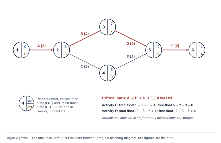
A network of six activities between six nodes, each node showing its number, earliest start time and latest finish time. Activity A, 3 weeks, runs from node 1 to node 2; Activity B, 4 weeks, runs from node 2 to node 3; Activity C, 2 weeks, runs from node 2 to node 4; Activity D, 5 weeks, runs from node 3 to node 5; Activity E, 3 weeks, runs from node 4 to node 5; Activity F, 2 weeks, runs from node 5 to node 6. The critical path is A, B, D, F, taking 14 weeks; its activities have no float. Activity C has a total float of 4 weeks and a free float of 0. Activity E has a total float of 4 weeks and a free float of 4.
Section 17: Key terms
Defined in the platform's own words. Each opens its full entry.
- Buffer stock HL
- The minimum level of stock a business plans to keep in reserve, so that it can keep producing or selling if a delivery is late or demand is higher than expected.
- Capacity utilization rate HL
- A business's actual output in a period as a percentage of its productive capacity, the most it could produce with its existing resources.
- Capital productivity HL
- The output produced per unit of capital used, such as per machine, per machine hour or per dollar of equipment.
- Capital-intensive production
- Production that relies more on machinery, equipment and technology than on people, so that capital is the largest share of its costs.
- Cost to buy (CTB) HL
- The total cost of buying a product or component from an outside supplier, instead of making it, for the quantity needed.
- Cost to make (CTM) HL
- The total cost of producing a product or component in-house for the quantity needed, made up of the fixed costs and the variable costs of production.
- Defect rate HL
- The percentage of units produced that fail to meet the required quality standard.
- Just-in-case (JIC) HL
- An approach to stock control that holds large stocks of materials and finished goods as insurance against late deliveries, faults or sudden rises in demand.
- Just-in-time (JIT) HL
- A lean method of production and stock control in which materials arrive just as they are needed and goods are made to meet actual orders, so that little or no stock is held.
- Labour productivity HL
- The output produced per worker, or per hour of labour, in a period.
- Labour-intensive production
- Production that relies more on people than on machinery, so that labour is the largest share of its costs.
- Lead time HL
- The time between placing an order with a supplier and receiving the goods, ready to use.
- Maximum stock level HL
- The highest level that stock is planned to reach, just after a delivery arrives.
- Operating leverage HL
- The extent to which a business's costs are fixed rather than variable, which decides how sharply its operating profit changes when its sales change.
- Outsourcing
- Paying another business to carry out an activity, or to make a product or part, that the business used to do, or could do, itself.
- Productive capacity HL
- The maximum output a business can produce in a period with the resources it has now, such as its buildings, equipment and staff.
- Productivity rate HL
- A measure of how much output a business gets from the inputs it uses, expressed as total output as a percentage of total input.
- Rationalization HL
- Reorganizing a business to cut costs and raise efficiency, often by reducing its capacity through closing sites, selling equipment or cutting staff.
- Reorder level HL
- The level of stock at which a new order is placed, set so that the delivery arrives before stock falls below the buffer level.
- Reorder quantity HL
- The amount of stock ordered each time a new order is placed.
- Spare capacity HL
- The extra output a business could produce with its existing resources, because it is producing less than its productive capacity.
- Stock control chart HL
- A graph of the level of stock over time, used to plan when to reorder and how much, showing usage, the reorder level, the lead time, the buffer stock and the reorder quantity.
- Stock-out HL
- A situation in which a business runs out of an item of stock, so that it cannot produce or cannot meet its customers' orders.
- Supply chain HL
- The linked sequence of organizations and activities that takes a product from raw materials, through production and distribution, to the final customer.
Section 18: Tools and practice
5 tools on the platform for 5.6, by room, with exercises, worked calculations and practice questions.
Advanced financial analysis
- Break-even scenarios Enrichment
Practice questions with mark schemes
Section 19: Check your recall
Answer from memory, then reveal and rate yourself. Your ratings stay on this device.
Answer each question from memory, out loud or on paper, before you reveal the answer. Your ratings also schedule these questions in your flashcards.
-
Give two advantages and two risks of a global supply chain.
Advantages, for example lower costs and access to materials or skills found elsewhere. Risks, for example long lead times, disruption from storms, conflict or pandemics, changes in exchange rates or tariffs, and harder checks on suppliers' ethics.
How well did you recall it? -
Why does just-in-time depend on reliable suppliers?
Because it holds little or no buffer stock, so one late or faulty delivery stops production.
How well did you recall it? -
A business uses 50 units a day, its lead time is 4 days and its buffer stock is 100 units. What is its reorder level?
100 + (50 × 4) = 300 units.
How well did you recall it? -
What is the difference between the reorder level and the reorder quantity?
The reorder level is the stock level at which an order is placed (when to order); the reorder quantity is the amount ordered each time (how much).
How well did you recall it? -
A factory can make 12,000 units a month and makes 9,000. What is its capacity utilization rate, and how could it raise it?
9,000 ÷ 12,000 × 100 = 75%. For example by boosting demand, using the spare capacity to make products for other firms, or rationalizing to cut capacity.
How well did you recall it? -
Of 1,500 units made, 45 fail inspection. What is the defect rate?
45 ÷ 1,500 × 100 = 3%.
How well did you recall it? -
Total contribution is $90,000 and fixed costs are $60,000. What is the degree of operating leverage, and what does it mean?
Operating profit is $30,000, so 90,000 ÷ 30,000 = 3. A 1% change in sales changes operating profit by 3%.
How well did you recall it? -
Give two reasons why a business might make a component even though its cost to make is above its cost to buy.
For example control over quality and supply, protecting its know-how, using spare capacity, or avoiding dependence on a single supplier or on suppliers with poor ethical standards.
How well did you recall it?
Section 20: How it connects
Where 5.6 meets the rest of the course: worked connections with an exam-style question on each, then the further links the notes name.
-
With 2.4 Motivation and demotivation
HR decisions and productivity HL
Labour productivity, output per worker or per labour hour, is where human resource decisions show up in operations. Training raises what each worker can produce; rewards and job design change how much effort people choose to give, which is the question the motivation theories try to answer, from Taylor's piece rates to Herzberg's motivators. High labour turnover works the other way: each leaver takes skills away, and recruiting and inducting a replacement costs time and money before the new worker reaches full productivity. The productivity measures belong to 5.6, so this connection is HL, but the link between motivation and output runs through the whole of Unit 2.
Exam-style question Source: Original practice question Command term: Explain (AO2)
Explain how two non-financial rewards could improve labour productivity in a business. [4 marks]
-
With 3.6 Efficiency ratio analysis
Stock turnover and just-in-time HL
Stock turnover measures how quickly a business uses or sells its stock: cost of sales divided by average stock gives the number of times a year, and average stock divided by cost of sales, times 365, gives the number of days stock is held. Just-in-time stock control sets out to hold as little stock as possible, with deliveries arriving as they are needed, so it raises stock turnover and frees cash that would otherwise sit in a warehouse. The price is exposure: with no buffer, a late delivery can stop production, which is why just-in-case stock remains the alternative.
Exam-style question Source: Original practice question Command term: Explain (AO2)
Explain how a move to just-in-time stock control might affect a business's stock turnover ratio. [4 marks]
-
With 5.7 Crisis management and contingency planning
Just-in-time and contingency planning HL
Just-in-time stock control holds almost no buffer stock, so it is efficient in normal times and exposed when something goes wrong: a late delivery, a fire at a supplier or a blocked port can stop production within hours. Contingency planning prepares for those failures in advance, for example by agreeing a second supplier, keeping a small buffer of critical parts or mapping the supply chain. Each measure adds cost and moves the business back towards just-in-case, which is why the impact of contingency planning has to be judged for the organization and situation in question.
Exam-style question Source: Original practice question Command term: Discuss (AO3)
Discuss the impact of contingency planning on a manufacturer that uses just-in-time stock control. [10 marks]
Also linked in the notes
- 3.7 Cash flow Stock ties up working capital, so stock control decisions affect cash flow.
- 4.3 Sales forecasting At HL, production planning, stock control and capacity utilization follow forecast demand.
- 5.1 Introduction to operations management At HL, capacity, stock control and the supply chain measure and manage how much an operation can produce.
- 5.2 Operations methods At HL, capacity utilization and productivity measure how fully and how efficiently a method's capacity is used.
- 5.3 Lean production and quality management Just-in-time is a lean production method, and the defect rate is what quality management sets out to cut.
- 5.4 Location Outsourcing, offshoring, insourcing and reshoring reshape the supply chain, and each is a decision to make or to buy on a larger scale.
- 5.5 Break-even analysis Contribution and the margin of safety underpin operating leverage, and capacity limits the output any break-even target can ask for.
- 5.9 Management information systems Real-time data from the internet of things and shared sales data support just-in-time stock control along the supply chain.
See 5.6 on the course connections map, with every link drawn across the five units.
Section 21: Connected learning
Everything else on the platform that teaches, applies or tests 5.6, each labelled by its standing.
- Revise
-
- The 5.6 mindmap Full and revision views, to print or download
- Revision sheet The subtopic on one printable page
- Flashcards The 5.6 cards, to rate as you go
- Practise
-
- 8 questions on 5.6 in the question bank From the practice sets, the notes and the case files, filtered to this subtopic
- Decisions and simulations
-
- Kestle Cycles: the cash runs out first Fictional Boardroom simulation
- Kilbrack Bakery: machines, people and the price of bread Fictional Boardroom simulation
- Hotel Mareluce: full rooms or a future Fictional Boardroom simulation
- Corvell Furniture: three years to restore the margin Fictional Boardroom simulation
- Frameworks
-
- Critical path analysis IB toolkitHL
- Tools
-
- 5 tools for 5.6 In Tools and practice on this page: Operations Floor, Advanced financial analysis
- Boardroom Briefings
-
- Kittiwake Air's margins fall for a third year Fictional Briefing 3
- Tasman Loaf Company weighs robots for its packing hall Fictional Briefing 4
- Tallowood Cafés is offered the roaster behind its coffee Fictional Briefing 8
- Business Intelligence
-
- The FCA closes its investigation into Drax's biomass statements without taking action Real-world A real development, 18 June 2026, with its sources
- Engine inspections keep Wizz Air jets on the ground as its annual profit falls to €1.3 million Real-world A real development, 11 June 2026, with its sources
- Kroger closes three automated warehouses built with Ocado and expects about $2.6 billion of charges Real-world A real development, 18 November 2025, with its sources
- Google's own AI chips reach a seventh generation, then an eighth Real-world A real development, 6 November 2025, with its sources
- Advanced Management
-
- Operations strategy, process optimization and lean systems Enrichment Operations and supply chain strategy: beyond the IB course
- Capacity planning, quality management and technology adoption Enrichment Operations and supply chain strategy: beyond the IB course
- Supply chain resilience, global sourcing and risk Enrichment Operations and supply chain strategy: beyond the IB course
- Course connections
-
- 3 worked connections on the connections map With 2.4, 3.6, 5.7
Notes checked against: Business management guide, first assessment 2024 (published February 2022, updated May 2022), pp. 34 to 35, 65 (The seven content statements and their assessment objectives; the capacity utilization and productivity rate formulas); Business Management for the IB Diploma, pp. 519 to 533 (Read to check coverage; nothing reproduced); Business management teacher support material, pp. 81 and 83 (The glossary's definitions of capacity utilization and the defect rate, checked). Updated 2026-11-03. The IB guide is the authority on the course.
Arjun Agrawal | The Business Brief, https://the-business-brief-dun.vercel.app/topics/production-planning/. Original teaching material, not an IB publication. The organizations in the teaching cases are fictional unless a case says otherwise.